Time as Scale: The Principle and Error Analysis of UWB TWR Two-Way Ranging

2026-09-22/ By Admin

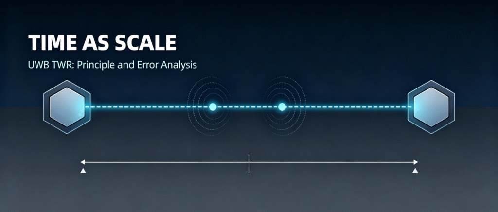
Why is it that the same "centimeter-level" UWB positioning can hit 10 cm in the lab, but drift to a meter or two in the field? Many engineers new to UWB indoor positioning hit the same wall: the TWR (Two-Way Ranging) principle looks simple enough, yet the distance error always comes out much larger than expected.

This article does not pile up formulas. It answers two things: what TWR actually measures, and where the error really comes from. By the end you will have a reusable framework for choosing a scheme and identifying error sources.

01 What exactly does TWR measure

The core idea of TWR (Two-Way Ranging) is straightforward: electromagnetic wave flight time grows with distance — the closer the nodes, the shorter the air time; the farther apart, the longer the propagation delay.

This relationship rests on the time-of-flight formula for UWB pulses:

d = c × ToF

where c is the speed of light and ToF is the signal flight time solved by the TWR algorithm.

Its biggest advantage is that the two nodes do not need clock synchronization. Each device runs on its own local clock; by exchanging question-and-answer frames and timestamps back and forth, the flight time is derived — which is exactly why TWR became the dominant ranging method for UWB indoor positioning.

But note: this formula stands on two ideal assumptions — line-of-sight propagation and perfectly accurate clocks. In reality, almost neither holds, and that is where the error begins.

02 Principle and derivation: from timestamps to distance

So far it has been intuition. This section works out the math of both schemes. Once you see how timestamps enter the formula, it becomes clear why error is inevitable and why it can be designed away.

SS-TWR timestamp arithmetic. Suppose the Tag sends a Poll at time T1, and the Anchor receives it at T2. After a fixed delay T_reply, the Anchor sends a Response at T3, and the Tag receives it at T4. The true one-way flight time ToF is:

ToF = ((T4 − T1) − (T3 − T2)) / 2

The corresponding distance is:

d = ToF × c

where c is the speed of light and ToF is the one-way flight time.

The logic: take the "total elapsed time (T4 − T1)", subtract the "Anchor processing time (T3 − T2)", and what remains is the net air time for a round trip; divide by 2 to get one way. No clock alignment between the two ends — that is the essence of TWR.

But the error hides in T_reply. The catch is that T1 and T4 are timestamped on the Tag clock, while T2 and T3 are timestamped on the Anchor clock. Two crystals can never run at exactly the same frequency. Let the Tag clock run fast by eA and the Anchor clock run fast by eB (in ppm); the measured round trip is then polluted by both clock biases, and the error magnitude is roughly:

ΔToF ≈ eA × ToF + (eB − eA) × T_reply / 2

where eA, eB are the relative crystal frequency offsets (ppm) of the Tag and Anchor, and T_reply is the Anchor-side response delay.

Note the second term: the error is proportional to the response delay T_reply. The longer T_reply and the larger the crystal frequency mismatch, the bigger the error. As a rough example (illustrative): with a 20 ppm frequency mismatch and 500 us response delay, (eB − eA) × T_reply / 2 is about 5 ns, roughly 1.5 meters. That is why SS-TWR is only suitable for short range and low-precision use cases.

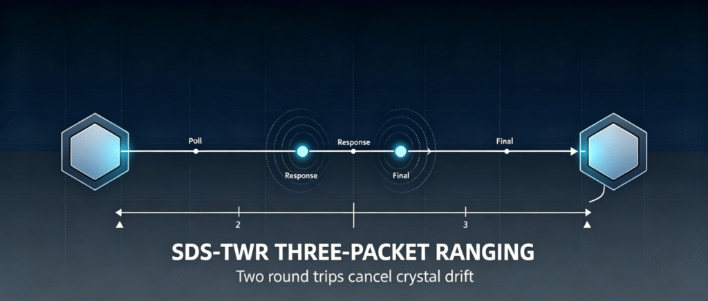
SDS-TWR and symmetric cancellation. SDS-TWR adds a third frame, Final: the Tag sends it at T5 (carrying T1 and T4 back to the Anchor), and the Anchor receives it at T6. This yields two independent round-trip measurements:

ToF1 = ((T4 − T1) − (T3 − T2)) / 2

ToF2 = ((T6 − T3) − (T5 − T4)) / 2

Taking the symmetric combination of the two as the final flight time:

ToF ≈ (ToF1 + ToF2) / 2

where ToF1, ToF2 are the flight times derived from the two round trips, and ToF is the combined result.

The key point: the two response delays are T_reply1 (Anchor side) and T_reply2 (Tag side). As long as each side keeps its own response delay fixed, the clock-bias terms cancel in the combination, leaving a residual error on the order of (eB − eA) × (T_reply1 − T_reply2). In practice the difference between T_reply1 and T_reply2 is far smaller than T_reply itself, so the error is typically more than an order of magnitude smaller than SS-TWR — the fundamental reason SDS-TWR is the high-precision choice.

Conclusion of the analysis. On the same RF hardware, the gap between two-packet and three-packet is not "a bit more data"; it shifts the dominant error term from "response delay × crystal mismatch" to "difference of response delays × crystal mismatch". Choosing SDS-TWR is essentially letting the clock errors of the two nodes cancel each other across two measurements.

03 Two mainstream schemes: pick the wrong one and the error balloons

There are two mainstream TWR implementations; distinguishing them first makes the later error discussion meaningful.

SS-TWR (Single-Sided Two-Way Ranging): only two frames are exchanged (Poll + Response). The algorithm is simple, air time is low, and power draw is small, but it has a fatal weakness — it cannot remove the error caused by crystal PPM drift. If the two clocks differ by even a few ppm, the ranging bias accumulates with distance; the farther you go, the worse it gets. It fits short-range, low-power, low-precision scenarios.

SDS-TWR (Symmetric Double-Sided Two-Way Ranging): three frames are exchanged (Poll + Response + Final), giving two round-trip measurements whose symmetry cancels the crystal frequency offset. It is the mainstream choice for high-precision indoor RTLS. The cost is one extra frame over the air, slightly more power and per-ranging latency.

One-line verdict: if you want precision, prefer SDS-TWR; reach for SS-TWR only when simplicity and low power matter more. But this is only the first step — choosing the right scheme does not by itself guarantee field accuracy.

04 Where the error comes from: three root-cause layers

Field error is never a single cause; it is the superposition of three layers. Troubleshoot layer by layer so you do not miss a key variable.

Layer 1, the physical layer. UWB is nanosecond pulses and is inherently sensitive to obstruction and multipath. Walls, metal cabinets, and human bodies all reflect or absorb the signal: reflection causes multipath superposition, tricking the receiver into picking the wrong first-arrival time; human blockage severely attenuates the signal or drops the direct path entirely (NLOS, non-line-of-sight). Inconsistent antenna polarization and phase offset also produce a fixed ranging bias. This layer is the "chassis" of error — if the physical environment is bad, no amount of upstream algorithm can rescue it.

Layer 2, the device and protocol layer. Crystal frequency offset and PPM drift are residual errors even SDS-TWR cannot fully remove; if antenna delay (the inherent circuit delay of the TX/RX chain) is not calibrated, you get a fixed bias on the order of tens of centimeters; when many nodes range at once, packet collisions in the air can make a ranging simply fail; jitter in the response delay injects noise into the timestamps. Problems at this layer are mostly solved by calibration and protocol design.

Layer 3, the model and environment layer. The TWR computation model is itself idealized; people walking and doors opening and closing make the environment dynamic; chip parameters drift with time and temperature; if the same board also runs WiFi and BLE, the 2.4 GHz coexistence interferes with UWB TX/RX. This layer determines how the error fluctuates.

Stack the three layers and you get a complete error chain: physical obstruction and multipath + clock and antenna error + model and environment fluctuation → wrong timestamps → wrong flight time → wrong distance. When troubleshooting in the field, work up this chain from the bottom and you will usually find the fastest path.

05 Common pitfalls: three assumptions worth questioning

Pitfall 1: "datasheet accuracy = field accuracy." The datasheet's centimeter-level number assumes line of sight, no multipath, and ideal clocks. Field acceptance must be measured in the real environment; do not take the datasheet number as the delivery target.

Pitfall 2: "SDS-TWR removes all clock error." What it removes is crystal PPM drift; it does nothing for multipath, NLOS, or antenna calibration bias. The algorithm is a tool, not a panacea.

Pitfall 3: "big error? add a filter." Filtering only smooths fluctuations; it cannot correct a systematic fixed bias. Check antenna calibration and physical deployment first, then talk about filtering.

06 A reusable framework for judging TWR schemes

Compress the whole article into a checklist to run through during selection and debugging:

When selecting: high precision with few nodes → SDS-TWR; short range, low power, low precision → SS-TWR; many concurrent nodes → confirm TDMA time-slot scheduling is supported.

When evaluating: use measured in-environment data for acceptance rather than datasheet specs; record the error distribution (P50/P90), not just the mean; keep edge data from multipath and obstruction scenarios as a statement of the system's capability ceiling.

One boundary to keep in mind: this framework holds in line-of-sight-dominated indoor environments. If the field is heavily obstructed, strongly multipath, and densely dynamic, UWB TWR alone will not deliver stable centimeter accuracy — you will need multi-source fusion or a different system architecture. That is not the algorithm failing; it is physics.

In the end, what separates one positioning system from another is never the chip’s nominal accuracy, but whether every step — physical deployment, protocol design, and data fusion — is done right. That is also the design philosophy behind SKYLAB’s UWB ranging modules, anchors, and tags.